The demand curve shows the amount of goods consumers are willing to buy at each market price.
A linear demand curve can be plotted using the following equation.
Qd = a – b(P)
- Q = quantity demand
- a = all factors affecting QD other than price (e.g. income, fashion)
- b = slope of the demand curve
- P = Price of the good.
Inverse demand equation
The inverse demand equation can also be written as
- P = a -b(Q)
- a = intercept where price is 0
- b = slope of demand curve
Example of linear demand curve
Qd = 20 – 2P

| Q | P |
| 40 | 0 |
| 38 | 1 |
| 36 | 2 |
| 34 | 3 |
| 32 | 4 |
| 30 | 5 |
| 28 | 6 |
| 26 | 7 |
| 0 | 20 |
Change in a
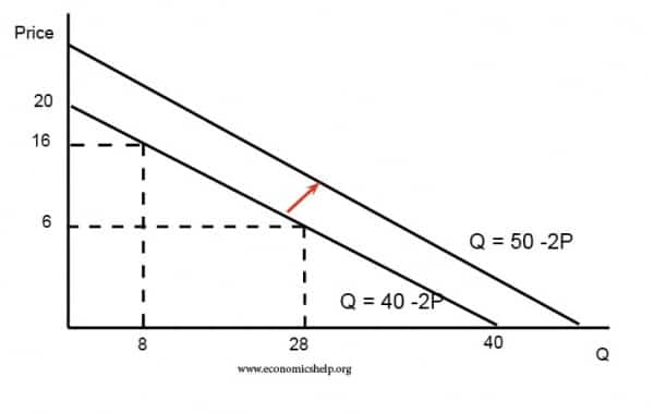
In this case, a has increased from 40 to 50.
This means that for the same price, demand is greater. It reflects a shift in the demand curve to the right. This could be due to a rise in consumer income which enables them to buy more goods at each price.
Change in b
In this case, the equation has changed from Q=40-2P to Q= 40-1P
This means the slope is steeper and looks like this.

Related
- Factors affecting demand
- Supply equation

Recent Posts
- UK Economic Decline During Past 100 Years
- How the Rich Avoid Paying Tax
- How Does Immigration Affect the Economy and Housing?
- Why UK Population Is Set to Fall Much Faster Than Forecast
- Why Denmark is rich despite high taxes?
Selected Posts
- Causes of Wall Street Crash 1929
- Causes of Great Depression
- UK economy in 1920s
- Keynesian Economics
- The problem of printing money
- The importance of economics
- Understanding exchange rates
- 10 reasons for studying economics
- Impact of immigration on UK economy
